Map Aggregation and Modeling

It is important to appreciate that the MaNGA datacubes exhibit significant spatial covariance between spaxels. For example, this is a critical consideration when binning spaxels to an expected S/N threshold; see Section 6 from Westfall et al. (2019, AJ, 158, 231).

The output quantities provided by the DAP are, therefore, also spatially correlated. The detailed calculation of covariance matrices for DAP quantities requires simulations that have not been performed! Having said that, some initial testing along these lines suggests that the correlation matrix of DAP quantities can be approximated by the nominal correlation between quantities in any given DRP wavelength channel.

Warning

The suggestions below are provided on a shared-risk basis, pending a more robust series of tests to validate this approach. Use with caution.

---

Approximate Correlation Between Spaxels

In Section 6.2 of Westfall et al. (2019, AJ, 158, 231), we showed that the correlation, \(\rho\), between spaxels as a function of the distance between them is well approximated by a Gaussian function.

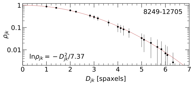
Figure 8 from Westfall et al. (2019, AJ, 158, 231): The mean (points) and standard deviation (errorbars) of the correlation coefficient, \(\rho_{jk}\), for all spaxels within the convex hull of the fiber-observation centers at channel 1132 (\(\lambda\) = 4700 Å) of datacube 8249-12705 as a function of the spaxel separation, \(D_{jk}\). The best-fitting Gaussian trend (red) has a scale parameter of \(\sigma\) = 1.92 spaxels, leading to the equation provided in the bottom-left corner.

You can construct the approximate correlation matrix for a given data cube as follows (cf. Spatial Covariance; Covariance):

from mangadap.datacube import MaNGADataCube
C = MaNGADataCube.from_plateifu(7815, 3702).approximate_correlation_matrix()

Initial tests suggest this correlation matrix is a good approximation for the DAP maps.

---

Approximate Covariance in a DAP Map

To construct the covariance matrix for a DAP map, start with the approximate correlation matrix and then renormalize to a covariance matrix using the provided variance data. For example, the following code constructs the covariance matrix in the \({\rm H}\alpha\) velocity measurements (note that the transposes are important; unfortunately, construction of the approximate correlation requires the instantation of the MaNGADataCube):

# Imports
import numpy
from astropy.io import fits
from mangadap.datacube import MaNGADataCube
from mangadap.dapfits import DAPMapsBitMask
from mangadap.util.fileio import channel_dictionary

# Read the datacube (assumes the default paths)
cube = MaNGADataCube.from_plateifu(7815, 3702)

# Construct the approximate correlation matrix
C = cube.approximate_correlation_matrix(rho_tol=0.01)

# Read the MAPS file
hdu = fits.open('manga-7815-3702-MAPS-HYB10-MILESHC-MASTARHC2.fits.gz')

# Get a dictionary with the emission-line names
emlc = channel_dictionary(hdu, 'EMLINE_GFLUX')

# Save the masked H-alpha velocity and velocity variance
bm = DAPMapsBitMask()
vel = numpy.ma.MaskedArray(hdu['EMLINE_GVEL'].data[emlc['Ha-6564'],...],
                           mask=bm.flagged(hdu['EMLINE_GVEL_MASK'].data[emlc['Ha-6564'],...],
                                           flag='DONOTUSE')).T
vel_var = numpy.ma.power(hdu['EMLINE_GVEL_IVAR'].data[emlc['Ha-6564'],...].T, -1)
vel_var[vel.mask] = numpy.ma.masked

# Construct the approximate covariance matrix
vel_C = C.apply_new_variance(vel_var.filled(0.0).ravel())
vel_C.revert_correlation()

---

2D Modeling of a DAP Map

When constructing a 2D model of the quantities in a DAP map, ideally you would account for the covariance between spaxels in the formulation of the optimized figure-of-merit. For example, with the covariance matrix, \({\mathbf \Sigma}\), the chi-square statistic is written as a matrix multiplication:

\[\chi^2 = {\mathbf \Delta}^{\rm T} {\mathbf \Sigma}^{-1} {\mathbf \Delta},\]

where \({\mathbf \Sigma}^{-1}\) is the inverse covariance matrix and \({\mathbf \Delta} = {\mathbf d} - {\mathbf m}\) is the vector of residuals between the observed data, \({\mathbf d}\), and the proposed model data, \({\mathbf m}\).

To fit a model then, we need to calculate the inverse of the covariance matrix. A minor complication in doing this for the DAP maps is that covariance matrix of the full map is always singular because of the empty regions in the map with no data. Taking care to keep track of original on-sky coordinates of each spaxel, we need to remove the empty regions of the map from the covariance matrix before inverting it. Continuing from the code above and assuming the masks for vel and vel_var mask out all spaxels without valid data:

# Flatten the map and get a vector that selects the valid data
vel = vel.ravel()
indx = numpy.logical_not(numpy.ma.getmaskarray(vel))

# Pull out only the valid data
_vel = vel.compressed()
_vel_C = vel_C.toarray()[numpy.ix_(indx,indx)]

# Get the inverse covariance data
_vel_IC = numpy.linalg.inv(_vel_C)

Assuming you have a vector with the model velocities (model_vel), you would then calculate \(\chi^2\) using the above matrix multiplication. Just for the purpose of illustration let’s set the model values to be 0 everywhere:

# Calculate chi-square
model_vel = numpy.zeros(_vel.size, dtype=float)
delt = _vel - model_vel
chisqr = numpy.dot(delt, numpy.dot(_vel_IC, delt))

Warning

Note that by definition \(\chi^2\) must be positive. However, a combination of the inaccuracies of the correlation approximation and numerical error in the inversion of the covariance matrix means that this would not necessarily be true in the example above. This is why I limited the construction of the approximate correlation matrix to require \(\rho \geq 0.01\); see approximate_correlation_matrix(). This is needed to ensure the calculation of chisqr above is positive, at least in the example case above.

---

Aggregation of Mapped Quantities

When aggregating data within a map, like summing within an aperture or calculating the mean within a region, propagation of the error aggregated quantity should account for spatial covariance. The easiest way to deal with the error propagation is to recast the aggregation as a matrix multiplication. The following is a worked example for binning the \({\rm H}\delta_{\rm A}\) index.

Warning

This example works with the uncorrected \({\rm H}\delta_{\rm A}\) index!

To start, here are the top-level imports:

# Imports
from IPython import embed
import numpy
from matplotlib import pyplot
from astropy.io import fits
from mangadap.datacube import MaNGADataCube
from mangadap.dapfits import DAPMapsBitMask
from mangadap.util.fileio import channel_dictionary
from mangadap.util.covariance import Covariance
from mangadap.util.fitsutil import DAPFitsUtil

Get the data

First, we extract the data, the weights needed to get the mean index, and the approximate covariance matrix. This is all very similar to what’s done to get the velocity measurements above:

# Read the datacube (assumes the default paths)
cube = MaNGADataCube.from_plateifu(7815, 3702)

# Construct the approximate correlation matrix
C = cube.approximate_correlation_matrix()

# Read the MAPS file
hdu = fits.open('manga-7815-3702-MAPS-HYB10-MILESHC-MASTARHC2.fits.gz')

# Get a dictionary with the spectral index names
ic = channel_dictionary(hdu, 'SPECINDEX_BF')

# Extract the masked HDeltaA index, its variance, and the relevant weight
bm = DAPMapsBitMask()
hda = numpy.ma.MaskedArray(hdu['SPECINDEX_BF'].data[ic['HDeltaA'],...],
                           mask=bm.flagged(hdu['SPECINDEX_BF_MASK'].data[ic['HDeltaA'],...],
                                           flag='DONOTUSE')).T
hda_wgt = numpy.ma.MaskedArray(hdu['SPECINDEX_WGT'].data[ic['HDeltaA'],...],
                               mask=bm.flagged(hdu['SPECINDEX_WGT_MASK'].data[ic['HDeltaA'],...],
                                               flag='DONOTUSE')).T
hda_var = numpy.ma.power(hdu['SPECINDEX_BF_IVAR'].data[ic['HDeltaA'],...].T, -1)

# Unify the masks (just in case they aren't already)
mask = numpy.ma.getmaskarray(hda) | numpy.ma.getmaskarray(hda_wgt) | numpy.ma.getmaskarray(hda_var)
hda[mask] = numpy.ma.masked
hda_wgt[mask] = numpy.ma.masked
hda_var[mask] = numpy.ma.masked

# Construct the approximate covariance matrix
hda_C = C.apply_new_variance(hda_var.filled(0.0).ravel())
hda_C.revert_correlation()

Construct a binning map

Just for demonstration purposes, we need to create a map that identifies the spaxels that will be aggregated. The following just constructs a rough, ad hoc binning scheme, with bins of roughly 3x3 spaxels:

def boxcar_replicate(arr, boxcar):
    """
    Boxcar replicate an array.

    Args:
        arr (`numpy.ndarray`_):
            Array to replicate.
        boxcar (:obj:`int`, :obj:`tuple`):
            Integer number of times to replicate each pixel. If a
            single integer, all axes are replicated the same number
            of times. If a :obj:`tuple`, the integer is defined
            separately for each array axis; length of tuple must
            match the number of array dimensions.

    Returns:
        `numpy.ndarray`_: The block-replicated array.
    """
    # Check and configure the input
    _boxcar = (boxcar,)*arr.ndim if isinstance(boxcar, int) else boxcar
    if not isinstance(_boxcar, tuple):
        raise TypeError('Input `boxcar` must be an integer or a tuple.')
    if len(_boxcar) != arr.ndim:
        raise ValueError('Must provide an integer, or a tuple with one number per array dimension.')

    # Perform the boxcar average over each axis and return the result
    _arr = arr.copy()
    for axis, box in zip(range(arr.ndim), _boxcar):
        _arr = numpy.repeat(_arr, box, axis=axis)
    return _arr

# Construct a binning array that bins all the data into 3x3 bins, with
# the bins roughly centered on the center of the map
nbox = 3
nmap = hda.shape[0]
nbase = nmap//nbox + 1
s = nbox//2
base_bin_id = numpy.arange(numpy.square(nbase)).reshape(nbase, nbase).astype(int)
bin_id = boxcar_replicate(base_bin_id, nbox)[s:s+nmap,s:s+nmap]

# Ignore masked pixels and reorder the bin numbers
bin_id[hda.mask] = -1
unique, reconstruct = numpy.unique(bin_id, return_inverse=True)
bin_id = numpy.append(-1, numpy.arange(len(unique)-1))[reconstruct]

Bin the data

By identifying which spaxels are in each bin, we can now construct the weighting matrix, bin the data, and get the covariance matrix of the binned data:

# Construct the weighting matrix
nbin = numpy.amax(bin_id)+1
nspax = numpy.prod(hda.shape)
wgt = numpy.zeros((nbin, nspax), dtype=float)
indx = numpy.logical_not(hda.mask.ravel())
wgt[bin_id[indx],numpy.arange(nspax)[indx]] = hda_wgt.data.ravel()[indx]
sumw = numpy.sum(wgt, axis=1)
wgt *= ((sumw != 0)/(sumw + (sumw == 0)))[:,None]

# Get the binned data and its covariance array
bin_hda = numpy.dot(wgt, hda.ravel())
bin_hda_C = Covariance.from_matrix_multiplication(wgt, hda_C.full())

We can then use reconstruct_map() to construct a map of the binned data with the same format as the original spaxel data, and create a plot that shows the two side-by-side:

# Reconstruct a map with the binned data
bin_hda_map = numpy.ma.MaskedArray(DAPFitsUtil.reconstruct_map(hda.shape, bin_id.ravel(), bin_hda),
                                   mask=bin_id == -1)

# Compare the unbinned and binned maps
w,h = pyplot.figaspect(1)
fig = pyplot.figure(figsize=(2*w,h))

ax = fig.add_axes([0.05, 0.1, 0.4, 0.8])
ax.set_xlim([2,38])
ax.set_ylim([3,39])
ax.imshow(hda, origin='lower', interpolation='nearest', vmin=-1, vmax=6)

ax = fig.add_axes([0.5, 0.1, 0.4, 0.8])
ax.set_xlim([2,38])
ax.set_ylim([3,39])
img = ax.imshow(bin_hda_map, origin='lower', interpolation='nearest', vmin=-1, vmax=6)
cax = fig.add_axes([0.91, 0.1, 0.02, 0.8])
cax.text(3., 0.5, r'H$\delta_A$ [${\rm \AA}$]', ha='center', va='center', transform=cax.transAxes,
         rotation='vertical')
pyplot.colorbar(img, cax=cax)
pyplot.show()

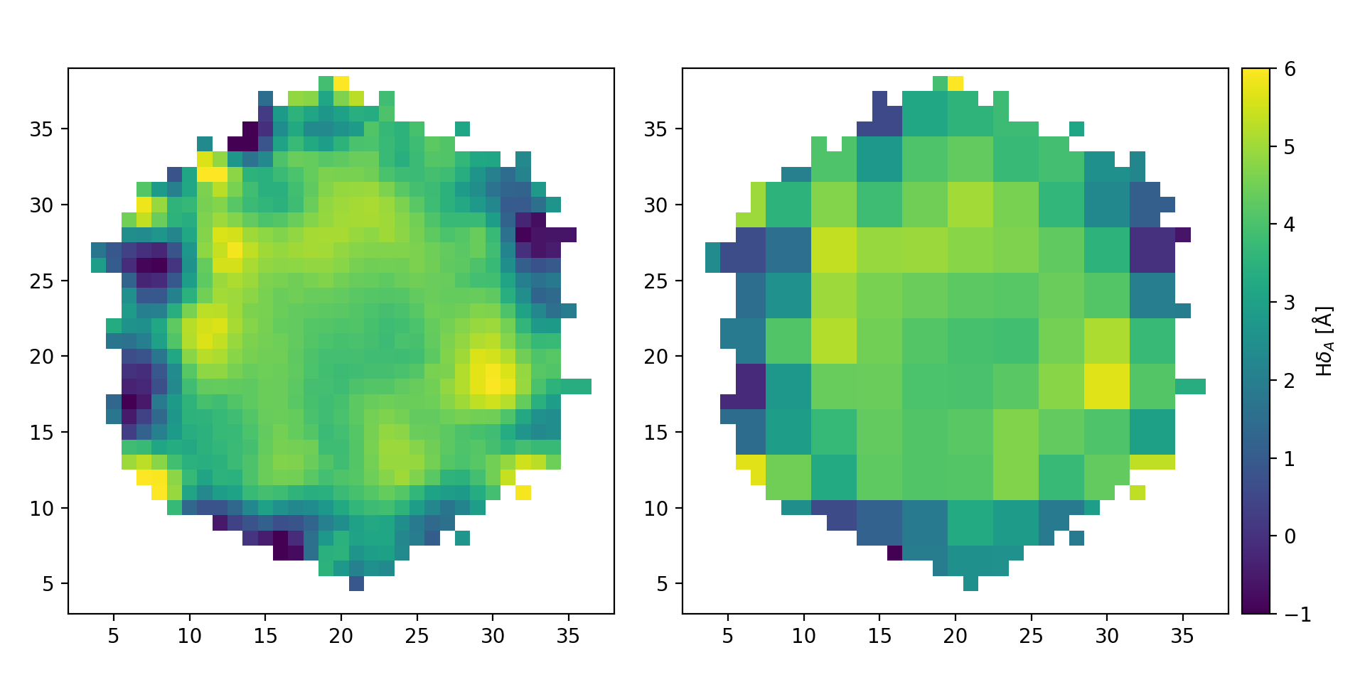
Comparison of the original \({\rm H}\delta_A\) map (left) with the result of binning the data in roughly 3x3 spaxel bins (right).

We can also compare the errors that we would have calculated without any knowledge of the covariance to the errors calculated using the approximate correlation matrix:

# Compare the errors with and without covariance
bad_var = numpy.dot(numpy.square(wgt), hda_var.ravel())
good_var = numpy.diagonal(bin_hda_C.toarray())

bad_sig = numpy.sqrt(bad_var)
pyplot.plot(bad_sig, 2.5*bad_sig, color='C3', zorder=1,
            label=r'$\sigma = 2.5 \sigma_{\rm no covar}$')
pyplot.scatter(bad_sig, numpy.sqrt(good_var), marker='.', s=80, color='k', lw=0, zorder=2)
pyplot.xlim([0,3])
pyplot.ylim([0,3])
pyplot.xlabel(r'$\sigma_{\rm no covar}$ [${\rm \AA}$]')
pyplot.ylabel(r'$\sigma$ [${\rm \AA}$]')
pyplot.legend()
pyplot.show()

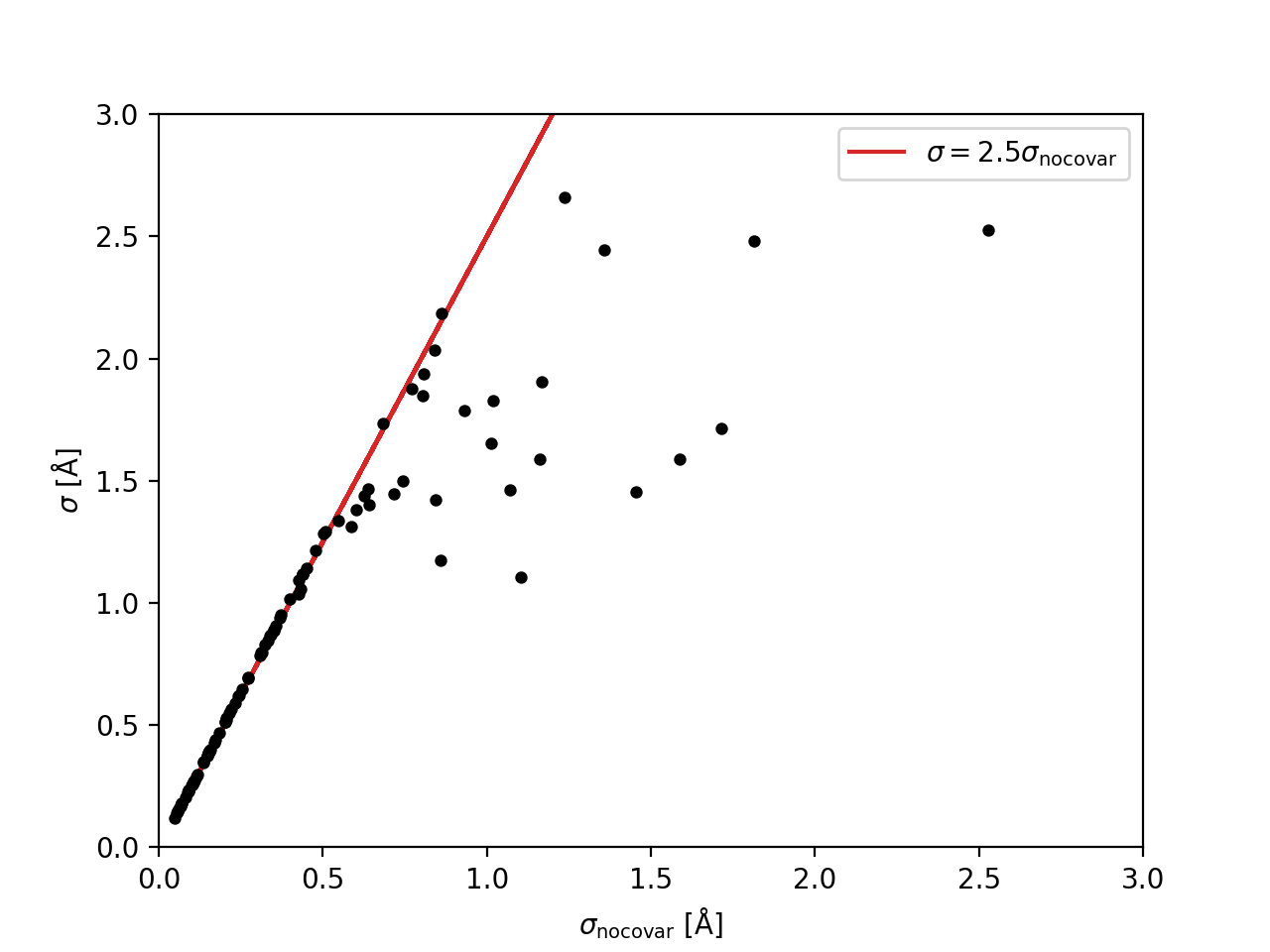
Comparison of the errors in the binned \({\rm H}\delta_A\) measurements without considering the covariance, \(\sigma_{\rm no covar}\), to the values that include the approximation of the covariance matrix, \(\sigma\). The red line shows that the errors that ignore covariance are underestimated by a factor of ~2.5.