Quality Assessment Plots
The DAP produces a number of quality assessment plots, ranging from those specific to the results of a given analysis module for a single observation to plots of global properties for all observations analyzed for a given MPL/DR. The QA plots are limited in many ways, but the following is a description of the current QA plots produced.
Warning
The file location and description below is specific to the MaNGA data. However, similar QA plots can be made for non-MaNGA data; see Execution.
Observation (PLATEIFU) specific
Spot-check MAPS
Script: $MANGADAP_DIR/bin/spotcheck_dap_maps
Output root: $MANGA_SPECTRO_ANALYSIS/$MANGADRP_VER/$MANGADAP_VER/[DAPTYPE]/[PLATE]/[IFU]/qa
Output file: manga-[PLATE]-[IFUDESIGN]-MAPS-[DAPTYPE]-spotcheck.png
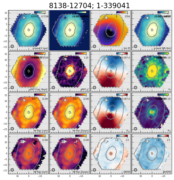
A selection of maps from the MAPS file for quick assessment of
the quality of the analysis. The PLATEIFU and MaNGA ID are
given at the top of the figure. The panels show from top-to-bottom
and left-to-right: \(g\)-band-weighted mean flux
(SPX_MFLUX), \(g\)-band-weighted spaxel S/N (SPX_SNR),
bin ID number (BINID), \(g\)-band-weighted bin S/N
(BIN_SNR), 68% growth of the fractional residual of the
stellar-continuum (kinematics) fit (STELLAR_FOM; channel
68th perc frac resid), \(\chi^2_{\nu}\) of the
stellar-continuum (kinematics) fit (STELLAR_FOM; channel
rchi2), stellar velocity (STELLAR_VEL), (uncorrected)
stellar velocity dispersion (STELLAR_SIGMA), non-parametric
\({\rm H}\alpha\) flux (EMLINE_SFLUX; channel
Ha-6564), Gaussian-fit \({\rm H}\alpha\) flux
(EMLINE_GFLUX; channel Ha-6564), ionized-gas velocity
(EMLINE_GVEL; channel Ha-6564), (uncorrected) \({\rm
H}\alpha\) emission-line velocity dispersion (EMLINE_GSIGMA;
channel Ha-6564), non-parametric \({\rm H}\beta\) flux
(EMLINE_SFLUX; channel Hb-4862), Gaussian-fit \({\rm
H}\beta\) flux (EMLINE_GFLUX; channel Hb-4862), D4000 index
(SPECINDEX; channel D4000), and the Dn4000 index
(SPECINDEX; channel Dn4000).
pPXF Results
Script: $MANGADAP_DIR/bin/dap_ppxffit_qa
Output root: $MANGA_SPECTRO_ANALYSIS/$MANGADRP_VER/$MANGADAP_VER/[DAPTYPE]/[PLATE]/[IFU]/qa
Output file: manga-[PLATE]-[IFUDESIGN]-MAPS-[DAPTYPE]-ppxffit.png
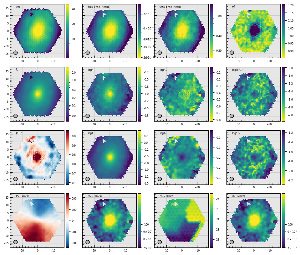
Metrics used to assess the results of the fit to the stellar
continuum performed by ppxf for the purpose of measuring the
stellar kinematics (see Stellar Kinematics). The plot
includes a few non-trivial metrics: \(A\) is the sum of the
absolute value of the additive polynomial coefficients,
\(A_n\) is similarly computed as \(A\) except that the
coefficients have been normalized by the mean \(g\)-band
weighted flux, and \(\delta A_n\) is the RMS of the polynomial
coefficients with respect to their median. The metrics denoted as
\(T\), \(T_n\), and \(\delta T_n\) are similarly
computed but using the template coefficients. These sets of
metrics are meant to provide a sense of how strongly the additive
polynomial coefficients and template mix vary across the galaxy.
Strong variations likely indicate artifacts in the spectra that
are throwing off the fit. The example shown here is typical. In
detail, the panels show from top-to-bottom and left-to-right: The
\(g\)-band-weighted spaxel S/N, the 68% and 95% growth of the
fractional residuals, the reduced \(\chi^2_{\nu}\), the
\(g\)-band-weighted mean flux, \(A\), \(A_n\),
\(\delta A_n\), the \(g-r\) color derived from the MaNGA
datacube (see the GIMG and RIMG extensions in the DRP
datacube), \(T\), \(T_n\), \(\delta T_n\), the stellar
velocity field, the “observed” (i.e., uncorrected) stellar
velocity dispersion field, the correction to apply to the stellar
velocity dispersion to account for the resolution difference
between the templates and the MaNGA spectra, and the corrected
(astrophysical) stellar velocity dispersion.
Full-spectrum fit residuals
Script: $MANGADAP_DIR/bin/dap_fit_residuals
Output root: $MANGA_SPECTRO_ANALYSIS/$MANGADRP_VER/$MANGADAP_VER/[DAPTYPE]/[PLATE]/[IFU]/qa
Output files:
manga-[PLATE]-[IFUDESIGN]-LOGCUBE-[DAPTYPE]-sc-fitqa-maps.png(left)
manga-[PLATE]-[IFUDESIGN]-LOGCUBE-[DAPTYPE]-el-fitqa-maps.png(right)
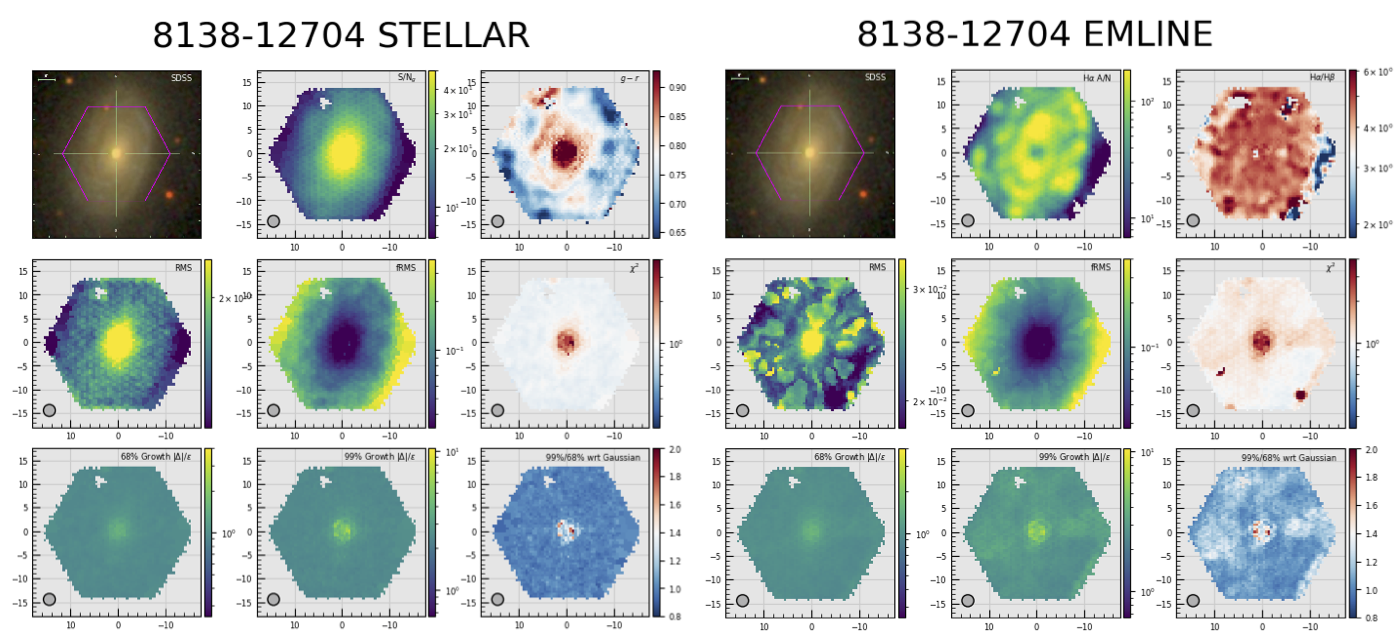
Maps used to assess the quality of the stellar continuum fits
(left) and the emission-line model fits (right). Left: The
maps in the first two rows, top-to-bottom and left-to-right, are:
the SDSS \(gri\) image with a purple hexagon outlining the
approximate size of the MaNGA IFU, the \(g\)-band-weighted
spaxel S/N, the \(g-r\) color derived from the MaNGA datacube
(see the GIMG and RIMG extensions in the DRP datacube),
the RMS of the fit residuals, the RMS of the model-normalized
residuals (i.e., the “fractional” RMS), and \(\chi^2_{\nu}\).
The bottom row shows, from left-to-right the 68% and 99% growth of
the error-normalized residuals and their ratio with respect to the
expectation of a Gaussian. If the distribution of the
error-normalized residuals strictly follow a Gaussian
distribution, the spaxesl in the left, middle, and right maps
should be 1, 2.6, and 1, respectively. Specifically for the
right-most image in the bottom row, spaxels below 1 have a
distribution of the fit residuals the falls more steeply than a
Gaussian, whereas values larger than 1 imply a more peaked
distribution (or at least one that has strong outliers). A more
direct view of the distributions relative to a Gaussian are shown
in the fitqa-growth plots below. Right: The maps in the
bottom two rows are the same as shown for the stellar-continuum
modeling. The middle and right-most plots in the top row, however,
are the amplitude-to-noise ratio of the \({\rm H}\alpha\) line
and the ratio of the \({\rm H}\alpha\) and \({\rm
H}\beta\) fluxes.
Output files:
manga-[PLATE]-[IFUDESIGN]-LOGCUBE-[DAPTYPE]-sc-fitqa-lambda.png(left)
manga-[PLATE]-[IFUDESIGN]-LOGCUBE-[DAPTYPE]-el-fitqa-lambda.png(right)
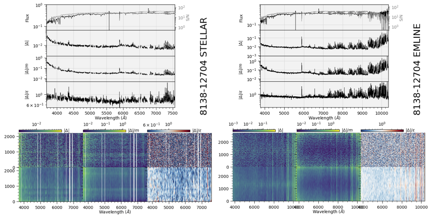
The left and right panel groups are identical; the left panels are for the stellar-continuum-fitting module and the right panels are for the emission-line-fitting module. Top: The top group panels show, from top-to-bottom, the flux and S/N (gray) averaged over all fitted spectra, the residuals averaged over all spectra, the model-normalized residuals averaged over all spectra, and the error-normalized residuals over all spectra. These plots aim to highlight any spectral regions that are poorly fit for all spectra, on average. Bottom: Two-dimensional maps of the residuals where wavelengths are ordered along the abscissa and the fitted spectra are organized along the ordinate; the value along the ordinate is the bin ID number. The residuals are shown twice, the top rows shows them at their native values (within the limits of the plot resolution) and the bottom smooths the data spectrally by 100 pixels. Masked regions are shown in white (e.g., emission-line regions in stellar-continuum fits in the left group). From left-to-right, the 2d images show the absolute value of the residuals (\(|\Delta|\)), the model-normalized residuals, and the error-normalized residuals.
Output files:
manga-[PLATE]-[IFUDESIGN]-LOGCUBE-[DAPTYPE]-sc-fitqa-growth.png(left)
manga-[PLATE]-[IFUDESIGN]-LOGCUBE-[DAPTYPE]-el-fitqa-growth.png(right)
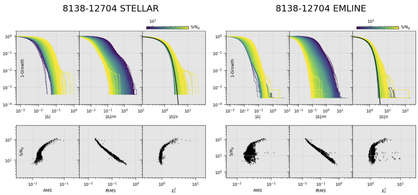
The left and right panel groups are identical; the left panels are for the stellar-continuum-fitting module and the right panels are for the emission-line-fitting module. Top: The top row of panels shows the growth curves (or actually \(1-g(x)\)) for the absolute value of the residuals, the model-normalized residuals, and the error-normalized residuals. One line is shown for each fitted spectrum; the lines are plotted from lowest to highest \({\rm S/N}_g\). In the right-most panel, the black line shows the expectation for a Gaussian error distribution. Bottom: From left to-right, the RMS of the absolute value of the residuals, the RMS of the model-normalized residuals, and \(\chi^2_{\nu}\).
Aggregated per plate
Script: $MANGADAP_DIR/bin/dap_plate_fit_qa
Output root: $MANGA_SPECTRO_ANALYSIS/$MANGADRP_VER/$MANGADAP_VER/[DAPTYPE]/[PLATE]/qa
Output file: [PLATE]-fitqa.png
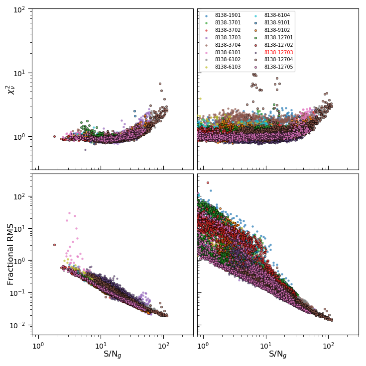
Each point in these plots is the result of a full-spectrum fit to
a single spectrum in either the stellar-kinematics (left column)
or emission-line-fitting (right column) modules. This plot
aggregates data from all observations on a given plate. The point
types for each plotted observation are shown in the legend.
Observations (PLATEIFU) numbers in red have been flagged by
the DRP as having critical data-reduction issues (CRITICAL).
Each panel shows a fit metric against the \(g\)-band S/N of
the spectrum. The top row shows the reduced chi-square and the
bottom row show the RMS of the model-normalized residuals. Compare
to Figure 27 from Westfall et al. (2019, AJ, 158, 231).
Aggregated per DAPTYPE
Script: $MANGADAP_DIR/bin/dapall_qa
Output root: $MANGA_SPECTRO_ANALYSIS/$MANGADRP_VER/$MANGADAP_VER/[DAPTYPE]/qa
Output file: dapall_radialcoverage.png
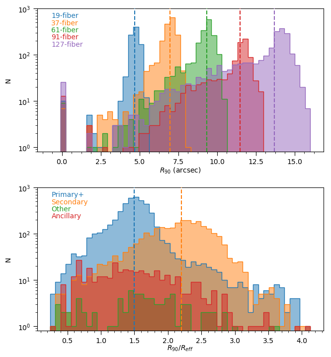
The radius to which at least 90% of a 2.5 arcsecond elliptical annulus is covered by spaxels analyzed by the DAP, \(R_{90}\). The top panel shows the distribution of \(R_{90}\) in arcseconds for observations taken with each bundle, colored by the bundle size. The bottom panel shows the distribution of \(R_{90}\) normalized by the elliptical-Petrosian half-light radius, \(R_{\rm eff}\), for galaxies belonging to the Primary+ and Secondary samples, as well as observations of ancillary or filler targets. Compare to Figure 28 from Westfall et al. (2019, AJ, 158, 231).
Output file: dapall_redshift_dist.png
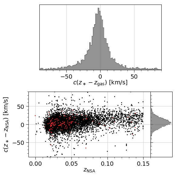
The comparison of the bulk redshifts from the NASA-Sloan Atlas
(NSA) and the bulk redshifts provided by the
DAPall database, where \(z_{\ast}\) is from the
STELLAR_Z column and \(z_{\rm gas}\) is from HA_Z. The
bottom-left panel shows the scatter plot (one point per
observations) with observations flagged as CRITICAL by the DRP
in red. The gray histograms only use data from datacubes that are
not flagged as CRITICAL.
Output file: dapall_mass_vel.png
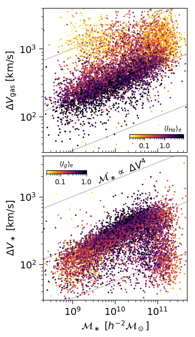
NSA stellar mass versus the velocity gradient—defined as \(\Delta V = (V_{\rm hi} − V_{\rm lo})/(1 − (b/a)^2)^{1/2}\), where \(V_{\rm hi}\) and \(V_{\rm lo}\) are provided by the DAPall file based on the emission-line (top) and stellar (bottom) kinematics. Points are colored according to the mean surface brightness within 1 \(R_{\rm eff}\). Compare to Figure 29 from Westfall et al. (2019, AJ, 158, 231).
Output file: dapall_mass_sigma.png
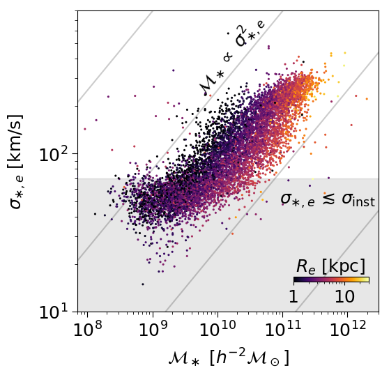
NSA stellar mass versus the light-weighted stellar velocity dispersion within 1 \(R_{\rm eff}\) from the DAPall file. Compare to Figure 30 from Westfall et al. (2019, AJ, 158, 231).
Output file: dapall_ew_d4000.png
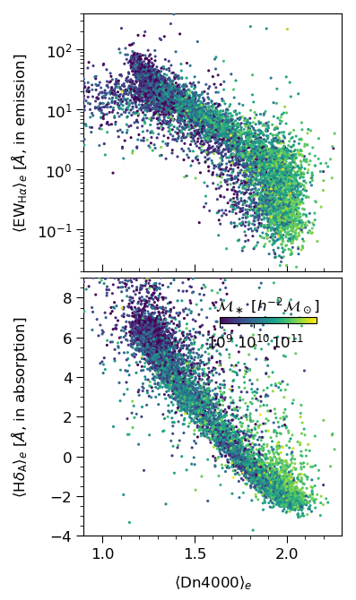
Dn4000 versus the \({\rm H}\alpha\) equivalent width in emission (top) and the \({\rm H}\delta A\) index (equivalent width in absorption) after subtracting the best-fitting emission-line model. Points are colored by the NSA stellar mass. Compare to Figure 31 from Westfall et al. (2019, AJ, 158, 231).
Output file: dapall_mgfe_hbeta.png
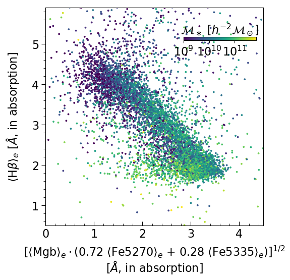
Typical stellar-population age–metallicity diagnostic using the Mgb, Fe5270, Fe5335, and \({\rm H}\beta\) absorption indices. Points are colored by NSA stellar mass. Compare to Figure 32 from Westfall et al. (2019, AJ, 158, 231).
Output file: dapall_mass_lha.png
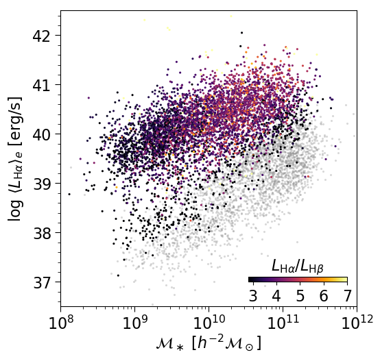
NSA stellar mass versus the absolute luminosity in \({\rm H}\alpha\). Points with \({\rm H}\alpha\) EW greater than 2 Å are colored by the \({\rm H}\alpha\)-to-\({\rm H}\beta\) luminosity ratio; others are set to gray. Compare to Figure 33 from Westfall et al. (2019, AJ, 158, 231).